Lab 05: Speed Control | Anuranan Bharadwaj

Experiment Overview

Speed control appears in nearly every powered system — jet engine fuel flow, electric motor drives, rotor RPM regulators, and propeller governor systems. The choice of controller architecture fundamentally changes how a system responds to step commands and rejects disturbances. This lab designed and directly compared two controllers for SRV02 motor speed regulation — a PI controller and a lead compensator — using both frequency-domain analysis (Bode plots) and time-domain step response evaluation in simulation and on hardware.

Analyze the stability margins of the augmented plant P_i(s) = K / [s(τs+1)] using Bode plots and gain/phase margin
Design and evaluate a PI controller for motor speed step tracking
Design and evaluate a lead compensator as an alternative controller architecture
Compare PI and lead performance in simulation and hardware implementation, explaining observed differences

Bode diagram of augmented plant Pi(s) – infinite gain margin, phase margin 87.8° at 1.53 rad/s — Figure 1: Bode diagram of P_i(s) — infinite gain margin, phase margin 87.8°

PI controller – simulated step response, tp=0.04 s, PO=4.4%, zero steady-state error — Figure 2: PI controller — simulated step response, t_p=0.04 s, PO=4.4%

Lead compensator – simulated step response, tp=0.04 s, PO=2.0%, zero steady-state error — Figure 3: Lead compensator — simulated step response, t_p=0.04 s, PO=2.0%

Equipment & Tools

Quanser SRV02 rotary servo-motor system
Q2-USB data acquisition board
VoltPAQ power amplifier
MATLAB/Simulink with QUARC real-time toolbox
MATLAB Control System Toolbox (margin() function for Bode analysis)

Frequency-Domain Analysis

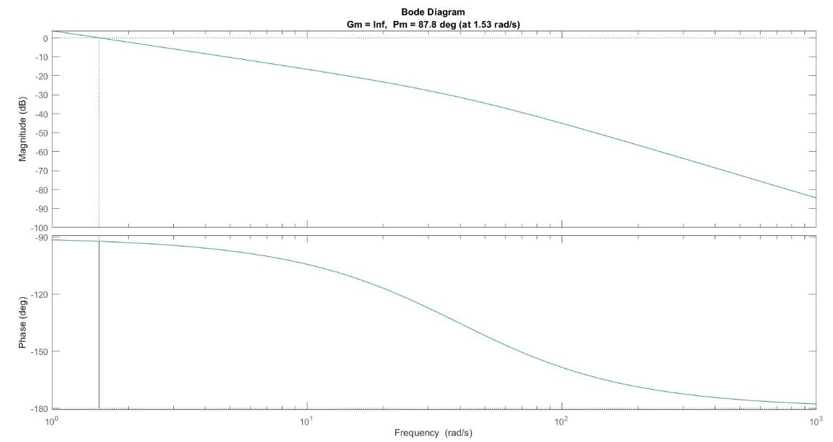
The plant including an integrator, P_i(s) = K / [s(τs+1)], was analyzed in frequency domain. The magnitude response is |P_i(jω)| = K / [ω√(1 + (τω)²)], which rolls off at −20 dB/decade from the origin pole, steepening to −40 dB/decade above ω = 1/τ = 39.4 rad/s. The phase starts at −90° and asymptotes toward −180° but never reaches it — giving the system an infinite gain margin. The phase margin was 87.8° at the gain crossover of 1.53 rad/s, indicating excellent stability robustness. Since one pole sits exactly at the origin, P_i(s) is marginally stable.

Key Results

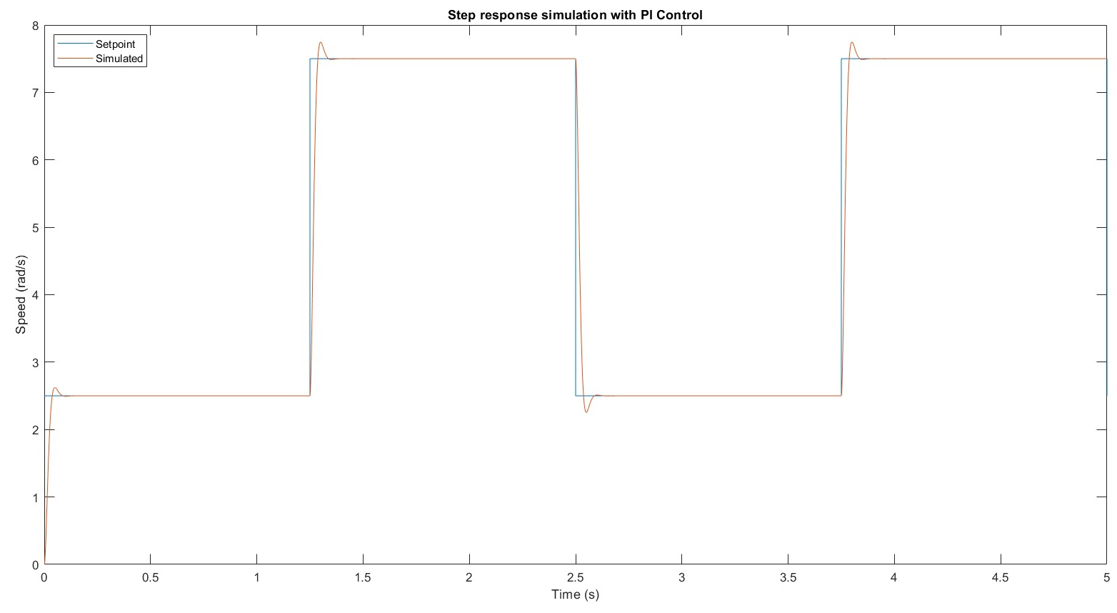
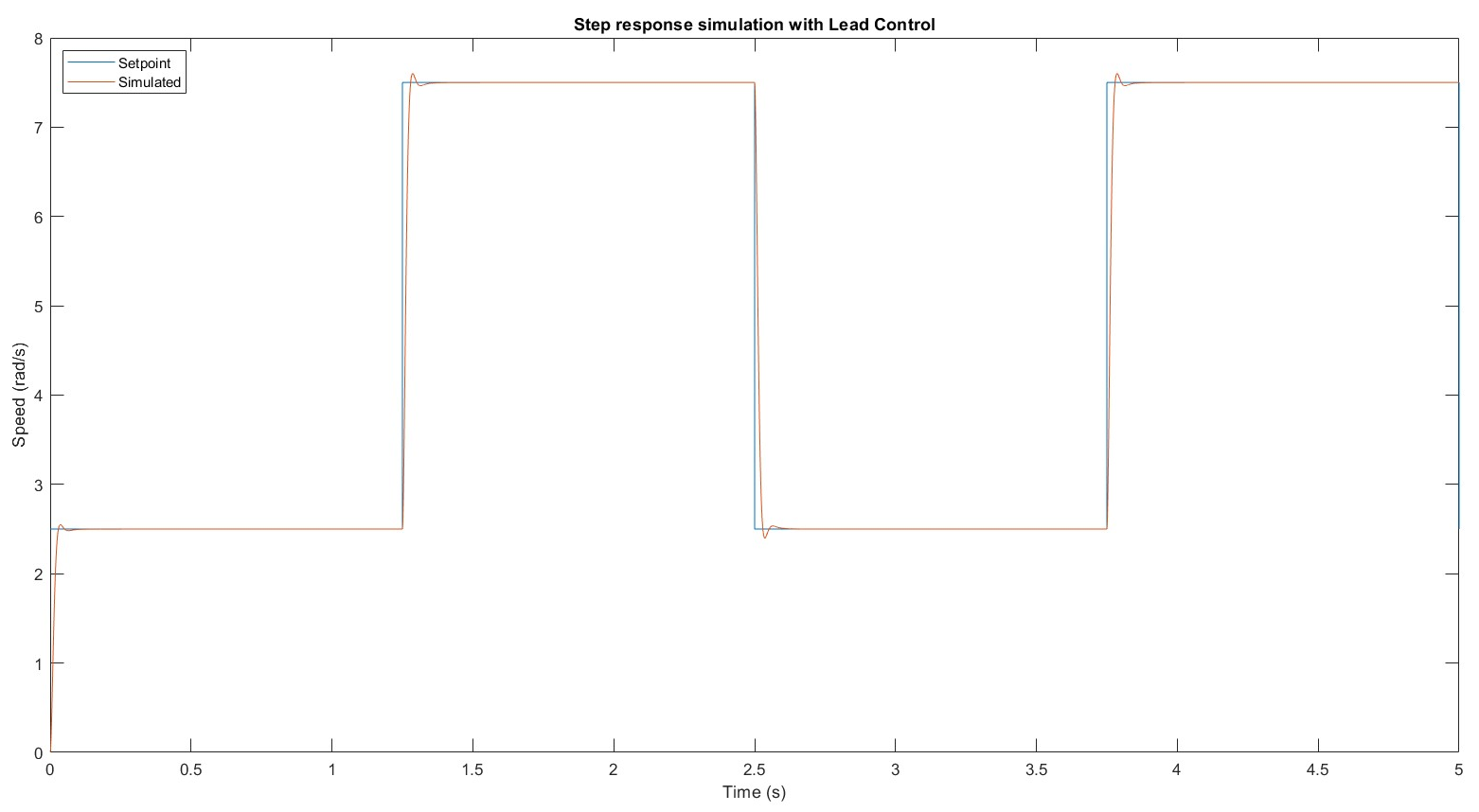
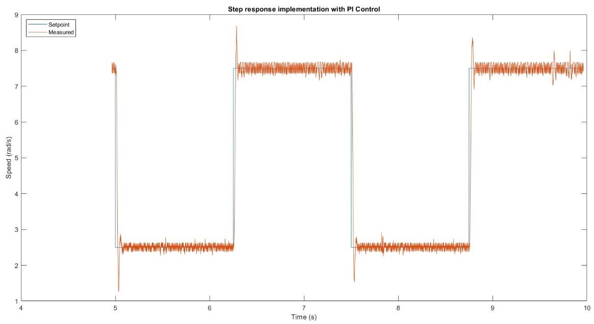
Controller / Test	t_p (s)	PO (%)	e_ss (rad/s)
PI — simulation	0.04	4.4	0
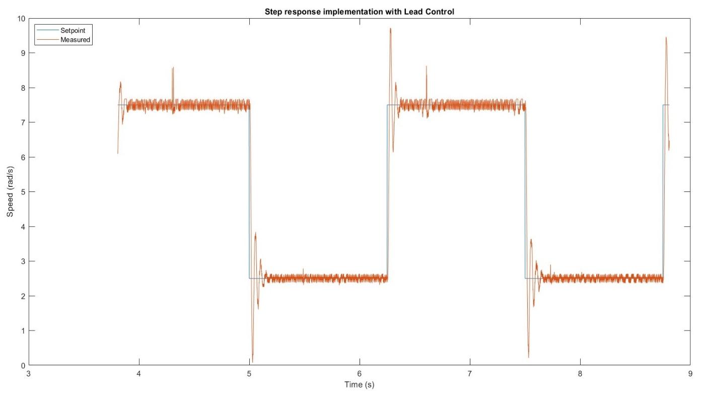
PI — hardware	0.034	23.8	−3.2 × 10⁻⁵
Lead — simulation	0.04	2.0	0
Lead — hardware	0.03	44.4	−0.0012

Both controllers met simulation specs; lead had marginally lower simulated overshoot (2% vs 4.4%).
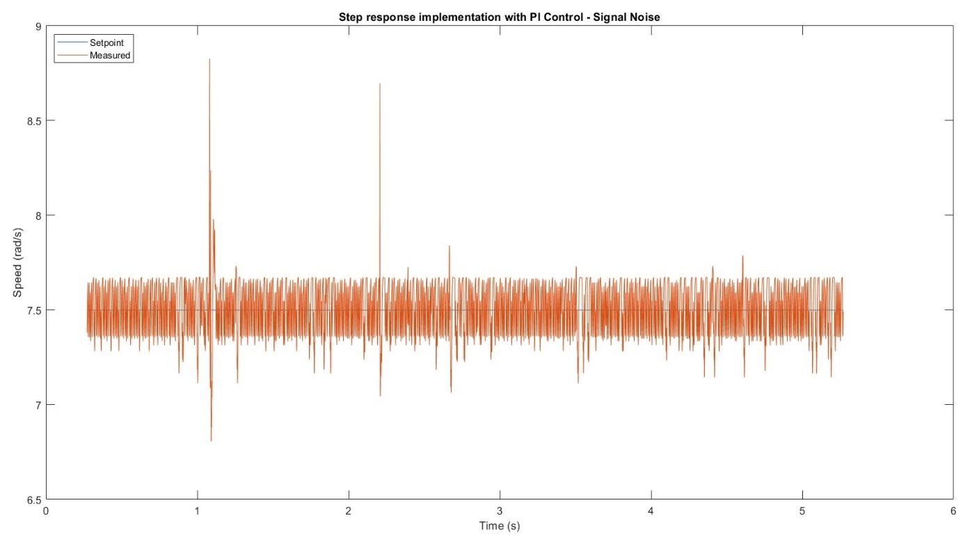
On hardware, PI overshoot (23.8%) was far more moderate than lead (44.4%) — the lead compensator’s derivative-like action amplified encoder quantization noise into the control signal, producing large velocity spikes at step transitions.
Measured PI peak-to-peak ripple: 1.16 rad/s vs. theoretical estimate of 0.525 rad/s — real encoder noise exceeded the theoretical bound, a practical insight about noise in digital velocity estimation.

PI controller – hardware step response, tp=0.034 s, PO=23.8% due to encoder noise — Figure 4: PI controller — hardware step response, PO=23.8%

PI controller – steady-state speed signal showing 1.16 rad/s peak-to-peak encoder noise ripple — Figure 5: PI controller — steady-state speed showing 1.16 rad/s encoder noise ripple

Lead compensator – hardware step response, PO=44.4% driven by derivative amplification of encoder noise — Figure 6: Lead compensator — hardware step response, PO=44.4%

MATLAB Code

The Bode plot was generated using MATLAB’s margin() function on the P_i(s) transfer function. Step response plots overlaid setpoint and measured speed, and steady-state error was computed over a time-averaged settling window.

% Augmented plant: Pi(s) = K / [s(tau*s + 1)]
K = 1.53;  tau = 0.0254;
s = tf('s');
Pi = K / (s * (tau*s + 1));
margin(Pi)    % Gm = Inf, Pm = 87.8 deg at 1.53 rad/s

% Step response overlay
plot(data_spd(:,1), data_spd(:,2))   % setpoint
hold on
plot(data_spd(:,1), data_spd(:,3))   % measured
xlabel('Time (s)');  ylabel('Speed (rad/s)')
legend('Setpoint', 'Measured')

% Steady-state error over settling window
index = (time >= 4.9) & (time <= 9.9);
e_ss  = mean(r(index)) - mean(y(index));  % ≈ -3.17e-5 rad/s (PI)

Valuable Takeaways

Simulation performance does not guarantee hardware performance. Lead looked better in simulation (2% vs 4.4% overshoot) but was significantly worse on hardware (44.4% vs 23.8%). Noise sensitivity that is invisible in a smooth simulation model becomes dominant when real encoder signals have quantization steps and electrical interference.
Frequency-domain stability margins tell you how much robustness you have. A phase margin of 87.8° means the plant can tolerate almost 90° of additional phase lag before going unstable — giving substantial robustness margin for real-world uncertainties in gain, delay, and model error.
Controller selection depends on the physical system, not just the model. For this servo application, PI was more practical than lead despite lead’s theoretical transient advantage, because PI is less sensitive to noise — a lesson that applies broadly to industrial motor drives and flight control actuators.
Completed the full frequency-domain control design cycle: Bode analysis → stability margin verification → controller synthesis → simulation validation → hardware implementation → performance characterization and explanation.